Overview

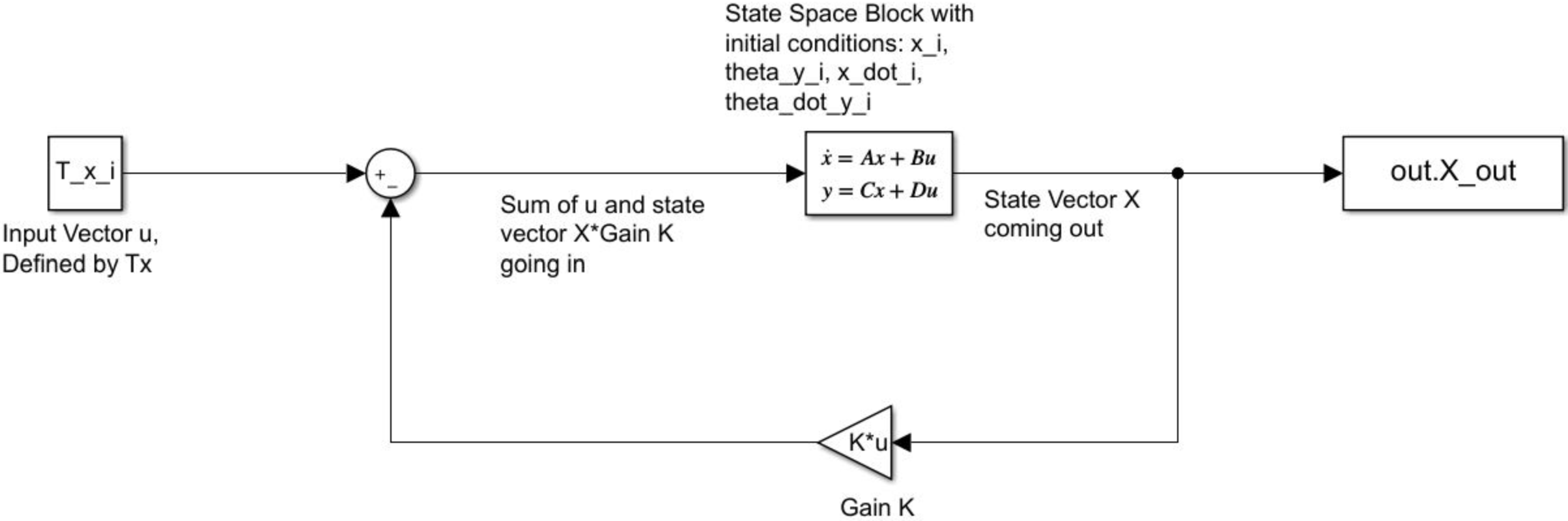
The goal of this assignment is to model the Equations of Motion derived in HW0x02 as a Linear State Space in the form of x_dot = Ax + Bu, where x is the state vector, A is the coefficient Matrix to the state vector, u is the input vector, B is the coeffcient Matrix to the input vector, and x_dot is the time derivative of the state vector x. In the context of the Equations of Motion representing the Ball-Plate system derived in Homework 2, the state vector would be a row vector of the position x, angle theta y and their derivatives, while the input vector is the torque output from the motor, and x_dot is the acceleration of the ball and the angular acceleration of the platform about the y axis. The implementation of this state space involved getting a matrix G that represented the matrix of accelerations from the inverse of the Mass Matrix M times the Forcing Function Matrix f. From there, the G matix was appended to a matrix h with x_dot (velocity) and theta_dot (angular velocity) as the first two elements in that matrix. The model was then linearized using Jacobian Matricies, which yielded A and B. From there, the Matricies A and B were implemented into a MatLab Simulink Model (see below) that calculated the output (position, angle, velocity and angular velocity) for both Open and Closed-loop controller set ups. Note the Gain for open loop is given as K = [0 0 0 0], and the Gain for closed loop was approximated to be K = [-0.3 -0.2 -0.05 -0.02] in the interest of evaluating system performance. Three test cases were used to verify the model's accuracy:

Open Loop, with all 0 initial conditions, running for 1 second.
Open Loop, with the only non-zero initial condition being x = 5 cm, running for 0.4 seconds.
Closed Loop, with the same initial conditions as Case 2 except T_x = -Kx, running for 20 seconds.

The Simulink Model used to generate output.

Case 1: Open Loop with Zero Initial Conditions

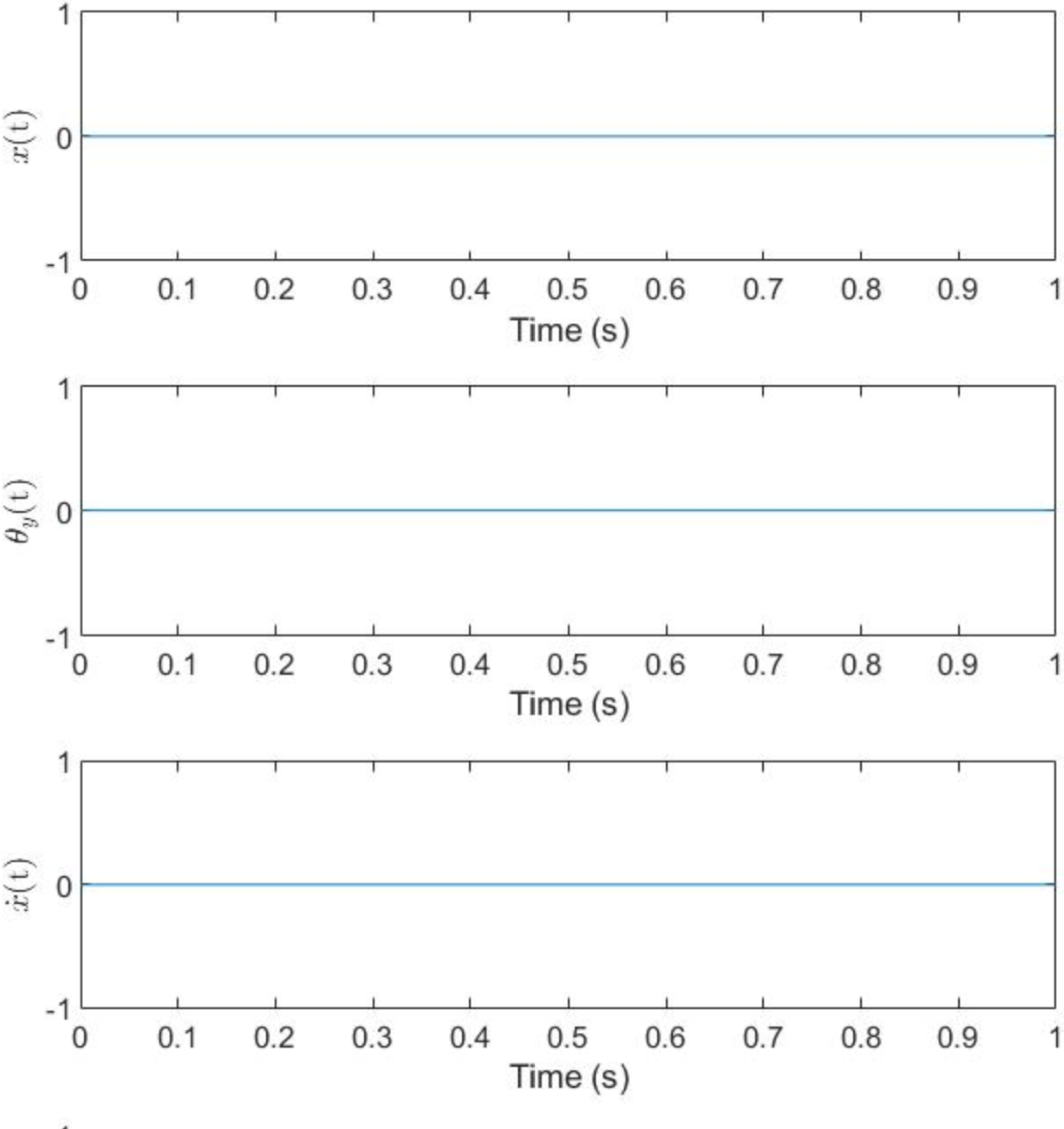
As one might expect from a system with zero initial conditions, there is no response in any element of the state vector. This acts as a sort of first "sanity check" that ensures no zero error occurs with no input in the model.

Case 2: Open Loop with x_i = 5 cm

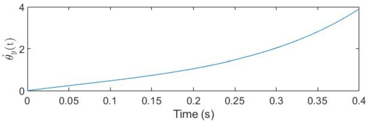
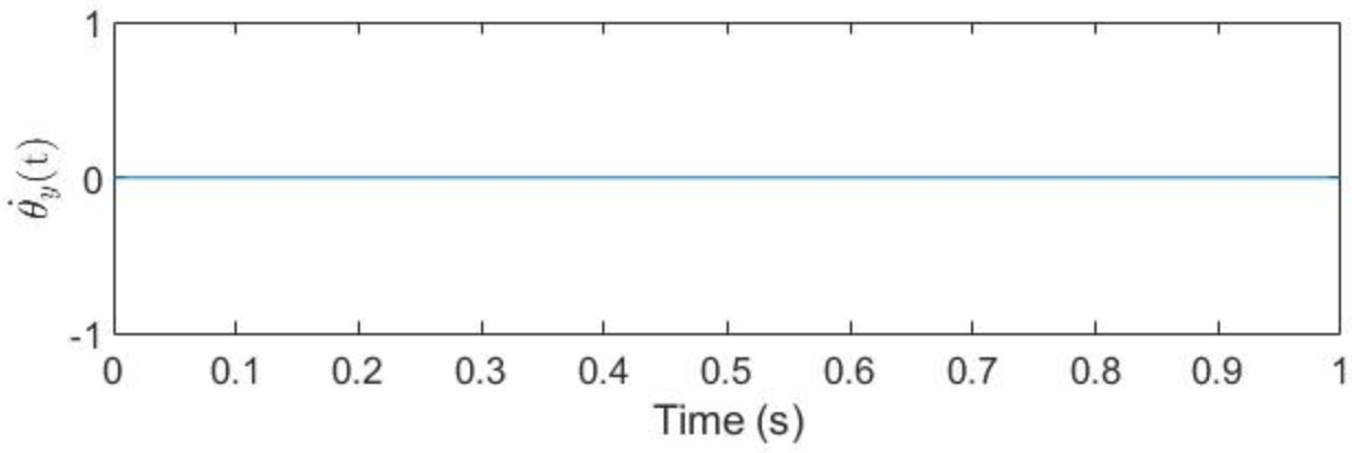
This acts as a second sanity check, where the ball starts 5 cm off the center of gravity of the platform with no torque input from the motor. The results are in agreement with what one would expect - that the platform begins to tilt due to the moment caused by the weight of the ball about the platform's center of rotation. The ball is shown to move towards the center a bit before rolling to the edge of the platform at an increasing velocity as the angle of platform tilt increases. With no torque input to correct this, the ball will simply roll off the edge at some time t in the future. Moreover, the ball moves barely more than a centimeter and reaches a velocity of just over 0.2 m/s, which makes sense given the short time frame and beginnng from rest - this validates the model for open loop responses from an intuition point of view.

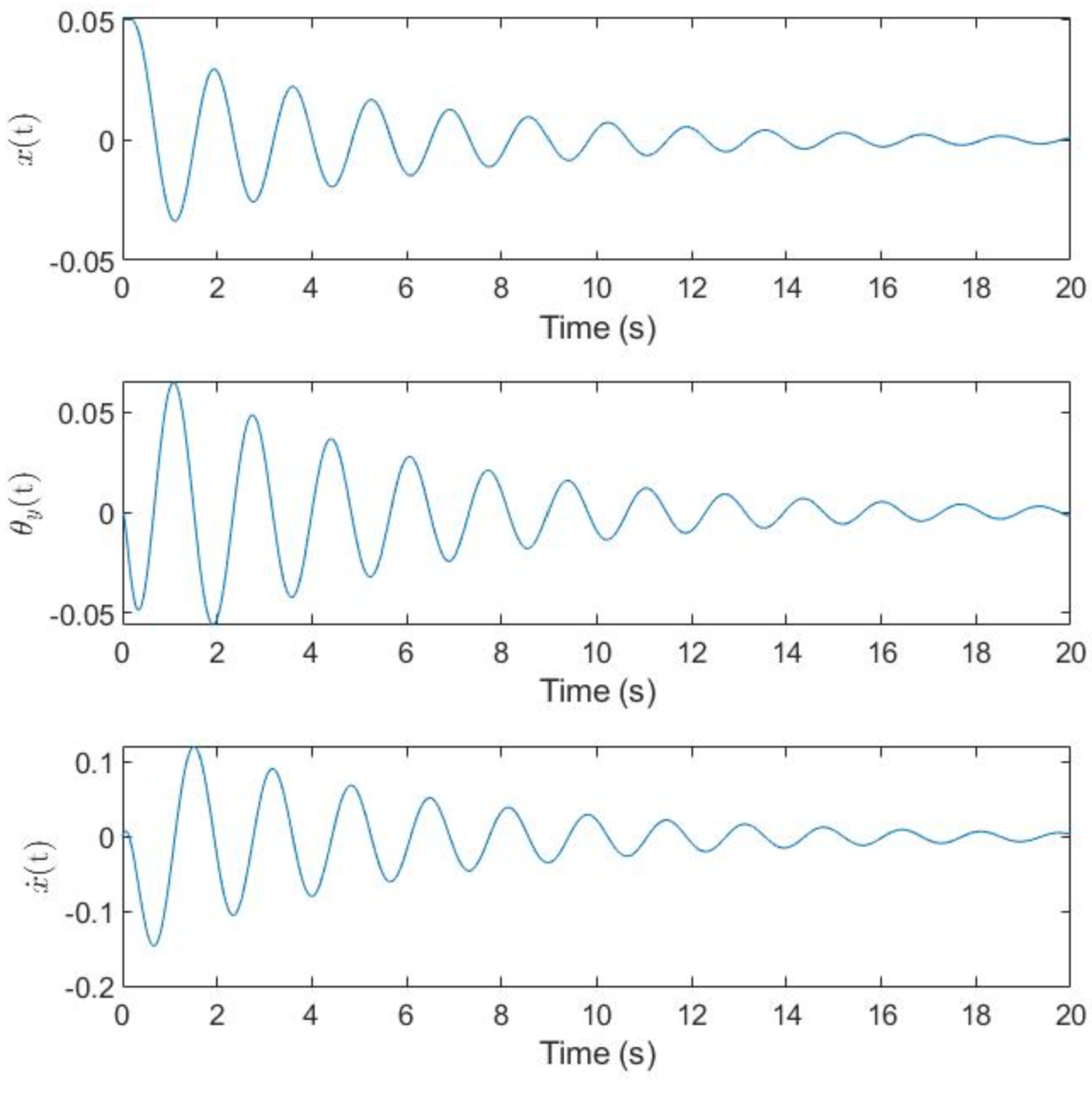
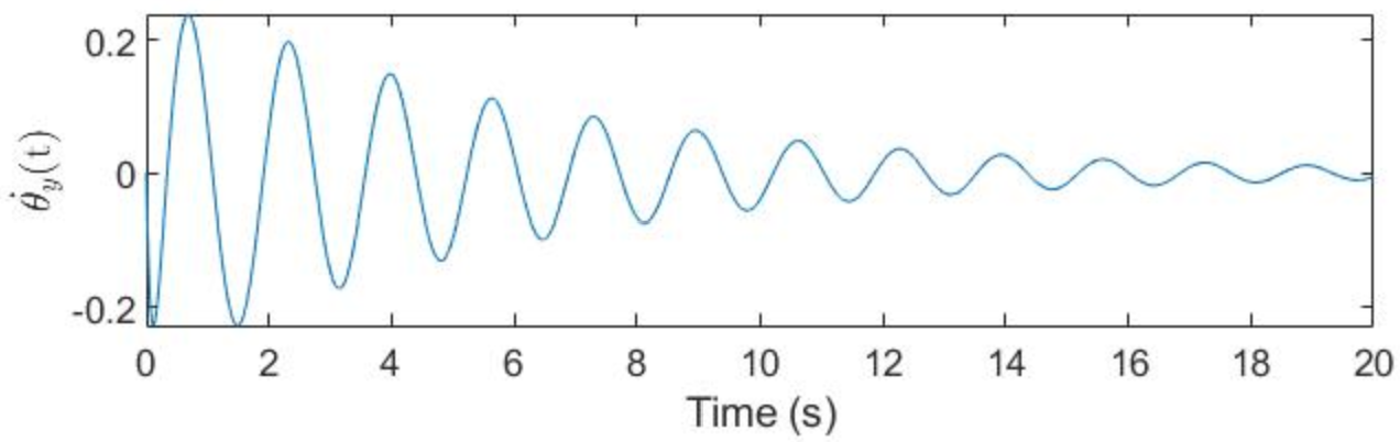
Case 3: Closed Loop with x_i = 5 cm and T_x = -Kx

Finally, we have a closed control loop with torque input from the motor and constant gain values. Note the gain values used are by no means ideal, which is why the system response takes roughly 15 to 20 seconds to reach steady state that is, the ball is balanced in the center of the platform. Otherwise, the output on the plots mostly agree with what makes sense with intuition. The ball oscillates from side to side on the platform as the platform moves to decrease the velocity of the ball and bring it back to a neutral position. As expected, the plots show a gradual decay in the magnitude of all state variables until they reach a steady state as the ball approaches the center of platform. Additionally, note the magnitude of the numbers makes sense, since the ball's position always decreases from 5 cm, while the platform's angle initially increases with every peak to compensate for the ball's rolling, but it eventually decreases as the ball's rolling becomes more controlled. Additionally, the ball's velocity never grows much beyond 0.1 m/s and the platform's angular velocity never gets larger than 0.2 seconds. These low numbers make sense for a system this small in scale, which validates the model's efficacy for Closed Loop Control.

Source Code

For the live Matlab script and Simulink Model, please visit this link: https://bitbucket.org/npatel68/me405_labs/src/master/hw4/

Author: Group 2: Neil Patel, Jacob Burghgraef

Date: May 9, 2021